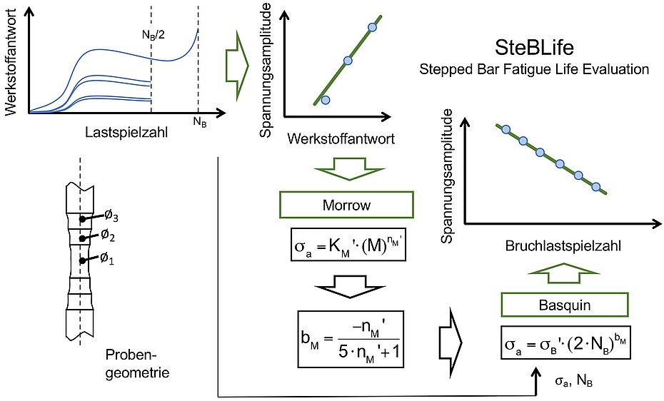
The fatigue tests are carried out at a constant force amplitude F_a or stress amplitude σ_a and the material response (MR) is recorded using various measuring methods. Due to the geometry of the specimen, 5 alternating deformation curves can be recorded simultaneously. The alternating deformation curves form the basis for the σ_a-MR correlations, which can be plotted and described shape-equivalent to Morrow [6]. Further, the Basquin relation [1] is used to calculate the Wöhler curve. This presented approach makes it possible to reduce the number of required tests to a few or even a single one, resulting in an enormous potential for the rapid verification of new materials and/or heat treatment processes. Thus, this procedure provides a valuable tool not only for basic research but also for applied research when it comes to developing new material concepts for a requirement-oriented material selection.

Following the SteBLife method, three different modules have now been developed and are currently in the validation phase on different unalloyed and low-alloyed carbon steels. The first module is SteBLife_stc(stc: single test, trend curve), which can be used to calculate a trend Woehler curve based on a single test with a time duration of 2-3 hours. SteBLife_mtc (mtc: multiple tests, trend curve) is based on the results of 3-4 SteBLife tests at different load horizons to improve the statistics of the underlying data set and provide a representative trend-Wöhler curve. The third module SteBLifemsb (msb: multiple tests, scatter bands) offers the possibility to calculate scatter bands for different failure probabilities, which can be of great interest for technical applications especially for more inhomogeneous materials like cast iron. For this purpose, 4-5 SteBLife tests are carried out on the same load horizon and the resulting fracture load cycles N_B are plotted over a Gaussian distribution. This makes it possible to determine failure load cycles for different failure probabilities such as P_f = 5 %, 50 % and 95 % (or others) [5].

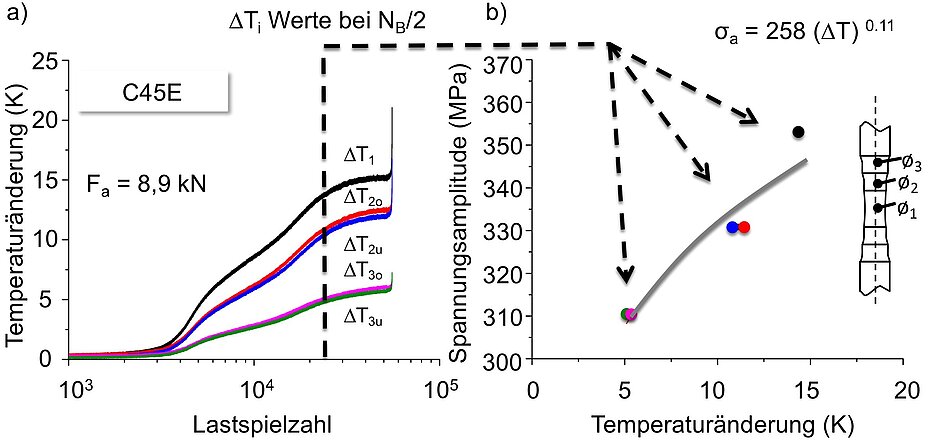
For the temperature measurements, seven measuring fields with 10 × 10 pixels each are defined along the specimen in the measuring software of the IR camera, one in each measuring length (T₁, T_2o/u, T_3o/u, o: top, u: bottom) and two at the clamping shafts (T_4o/u), whereby the temperature change ΔT is formed as the difference temperature from the individual specimen areas [5]. The diameters of the specimen shafts are much larger than those of the test sections, so that T_4o/u contains only elastic deformation components and temperature effects from the environment. T_4o/u is therefore subtracted fromT₁, T_2o/u, T_3o/u, resulting in the temperature changes ΔT₁, ΔT_2o/u, ΔT_3o/u, which in turn can be qualitatively assigned to the local plastic deformations in the various gauge lengths.

For SteBLifem_sb, a total of 5 tests were carried out with a sinusoidal loading and a force amplitude of F_a = 8.9 kN at a load ratio of R = -1. Due to the symmetry of the specimen geometry, one alternating deformation curve for the test section diameter 6 mm and two each for the test section diameters 6.2 and 6.4 mm can be recorded simultaneously at local stress amplitudes of 352 (T₁), 329 (T_2,o/u) and 309 MPa (T_3,o/u), respectively (Fig. 3a).

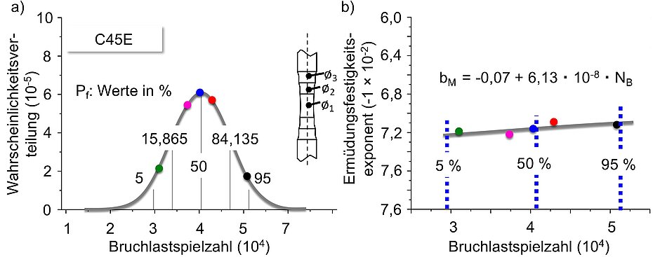
Following the SteBLife_msb approach, the results of the 5 tests carried out are analyzed with respect to the number of cycles NB and the sa-NB relationship (Fig. 4). Both N_B and the σ_a-N_B relationship show scatter, which can be attributed to material inhomogeneities, among other things.

According to the Gaussian distribution, N_B can be determined for different probabilities of default P_f. In this example, P_f = 5, 50 and 95 % was chosen to represent the scatter bands. From the 5 SteBLife tests, various fatigue strength exponents b_M (see Fig. 2) can also be determined and plotted as a b_M-N_B relationship depending on the number of fracture load cycles. Using the N_B calculated for P_f = 5, 50 and 95 % (Fig. 4a) in the b_M-N_B correlation (Fig. 4b), corresponding b_M values for the relevant failure probabilities can also be derived (Fig. 4b).

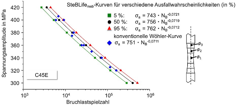
Based on the calculated N_B and b_{M v}alues, the Wöhler curves are then calculated with scatter bands for P_f = 5%, 50% and 95%. The results are shown in Fig. 5 together with the fracture load cycles of 11 ESV performed with conventional Hourglass specimens.

Fig. 5 illustrates that the conventionally determined service lives can be reliably described by the scatter bands calculated on the basis of SteBLife_msb. The fatigue strength coefficients and exponents of the calculated and conventionally determined Wöhler data are in the same value range.